Probability Distribution Definition
In statistics and probability theory, a probability distribution is defined as a mathematical function that describes the likelihood of all the possible values that a random variable can assume within a given range. This range is bounded by minimum and maximum possible values.
Probability distributions indicate the likelihood of the occurrence of an event or an outcome. It tells us whether our data sets is continuous or discrete. Gaussian or Exponential. Univariate or multivariate. What each of those terms are will be studied in detail later but for now understand that there are different types of distributions based different types and nature of data.
For example, take the outcome (X) of coin tossing as an experiment. When you toss the coin once or twice, there is no way for you to say with a surety if you will land a heads or a tails next. But take a long enough timeline of thousand or ten thousand tosses and the probability distribution of X would be 0.5 for heads and 0.5 for tails. This tells us a lot about the possible outcomes and it’s distribution.
Likewise, you can learn a lot about different probability distribution patterns for other simple events like picking a card, heights of men and women, weather and other data. But the real use of these probability distributions is when you use it to understand much more complex data and patterns in different fields of life making it a very useful tool in data science & statistics. Probability distribution helps us understand the spread of potential values, predict missing values, likelihood of outcomes and other results. It is an quintessential tool when it comes to big data and data science.
Ways of Displaying Probability Distributions
Before we proceed ahead and understand probability distributions in detail, first let us study the different ways in which a probability distribution is displayed.
Probability Distributions can be displayed in three ways:
a. Graphs: Most of the statisticians usually prefer using graphs over tables/formulas due to how easily it conveys the probability distribution at hand. Statisticians don’t restrict themselves to graphs rigidly and will use tables and equations wherever necessary. Take for example one of the most common types of distribution used in statistics which is the standard normal distribution.
A graph like this helps conveying and making sense of a lot of data succinctly. Similarly, graphs are also very helpful when it comes expressing the differences between continuous probability distributions versus discrete probability distributions and the different types of each which we will study in detail later below.
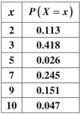
b. Tables: Sometimes the probability distribution at hand is better expressed in a tabular form. Take for example the below probability distribution where column two denotes the likelihood of occurrence of values in column one. Note the sum of all the probabilities is equal to 1 (.113+.418+.026+.245+.151+.047 = 1)
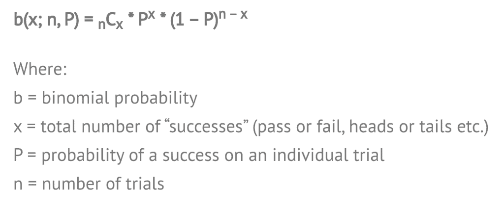
c. Formulas: The same distributions can also be expressed as formulas or equations. For example, the binomial distribution although expressed both as a graph and as a formula is often used as a formula more. Don’t worry what the binomial distribution is for now, we will understand it in detail later.
Types of All Probability Distributions in Statistics
Before listing all the various probability distributions in statistics, let us first understand the big broad bifurcations of the types of probability distributions in statistics namely: Discrete Probability Distributions and Continuous Probability Distributions
Discrete Probability Distributions
Discrete probability distributions are probability distributions where the variables are discrete. The word ‘Discrete’ in simple language means individually separate and distinct. Hence, distributions in which the random variable is discrete, that is individually separate and distinct, will have a discrete probability distribution.
To understand what discrete functions mean, take for example the count of number of students in a classroom. You will get values like 10, 12, 15 or 50 students but not decimal or fractions in between like say 22.45. Or take for example the coin toss, where the only outcomes are either heads or tails and nothing in between. These are examples of discrete functions.
Discrete probability functions are also known as probability mass functions. A discrete probability distribution can take a countable number of values. In cases where the range of values is countably infinite, these values have to decline to zero fast enough for the probabilities to add up to 1. Meaning the sum of probabilities 1/2 + 1/4 + 1/8 + … = 1
For example, take a hypothetical example of the probability of the number of houses owned by men under 50 in a local county. The sum of all the probabilities in this case would be equal to one 0.31+0.43+0.19+0.07=1
| Number of Houses Owned | Probability |
| 0 | 0.31 |
| 1 | 0.43 |
| 2 | 0.19 |
| 3 | 0.07 |
Types of Discrete Probability Distributions
There are different types of discrete probability distributions which differ based on the different types and properties of data. For example, a binary data like the heads and tails of a coin toss differs a lot from the kind of data of rolling a die and will have different types of discrete probability distributions
- Binomial distributions: In the above example of a coin toss, the only two outputs are head or tail. In such a distribution, where the distribution is binary, the discrete probability distribution is said to be a binomial distribution. Binomial data has further types like hypergeometric, negative binomial distribution and geometric distribution.
- Uniform distribution: Uniform distribution are the kind of distributions where multiple outcomes have the same probability. For example, in the above rolling a die case, each output has an equal probability of 1/6. Such a discrete probability distribution is said to be uniform in nature.
- Poisson distribution: A Poisson distribution is a type of discrete probability distribution which the probability of a given number of events occurring in a fixed space of time interval but can also be used to measure number of events in specified intervals of area, volume and distance. For example, take the example of number of people buying apples in between 6.30 pm and 7.30 pm in a grocery store during weekdays. Such a distribution would be a Poisson distribution
We will take a look at some of these types and more, in detail later.
Finite support vs infinite support: Another important characteristic when it comes to types of discrete probability distributions is finite vs infinite support. Let’s have a look in more detail about each of these types.
- Finite support: When a discrete probability distribution is said to have finite support, it means that the discrete distribution can only have a finite number of possible outcomes. Like in the coin toss example that we talked above, the only two outcomes are either a ‘Head’ or a ‘Tail’ and such a discrete distribution is said to have finite support.
- Infinite support: Whereas for a discrete probability distribution with infinite support, it can have an infinite number of possible outcomes. Take for example, the number of people buying a product on Fridays. The values can be 0,1,2,3, … right up to infinity. Such a discrete distribution is said to have infinite support.
Continuous Probability Distributions
Continuous probability distributions are probability distributions where the variables are continuous and not discrete. Meaning, in a continuous distribution the variable can both: (1) Assume an infinite number of values between any two values, and (2) Specific values can have a zero probability unlike discrete distributions where each value has a non-zero likelihood.
For example, in contrast to a coin toss where the only two discrete outcomes are ‘Head’ or ‘Tail’, a continuous probability distribution like the heights, weights or weather can have an infinite number of values. We can record the temperature every day and it can be a different value. The probability that the temperature is exactly the one predicted on a given day is close to zero.
Continuous probability distributions are also known as probability density functions. Just like the differences in discreteness of data leads to different types of discrete probability distributions, similarly for continuous probability distributions, the variations in the type of continuity and the shapes of the distributions get affected a lot by the variability and nature of the data accounted for.
Most continuous distributions have a few key parameters that majorly affect how the distribution is shaped. Few of the most commonly known and used distribution patterns like the Normal Distribution or the lognormal distribution are shaped uniquely based on these key parameters. For example, in the normal distribution the ‘mean’ and ‘the standard deviation’ are few of the key parameters which shape the data.
We will take a deeper look at each of these types of continuous probability distributions in depth later.
Further Types of Continuous Probability Distributions: Just like the discrete probability distributions which are categorised with finite or infinite support, similarly continuous probability distributions are also categorised with their support.
Namely the continuous probability distributions are categorised as:
- Supported on a bounded interval
- Supported on intervals of length 2π – directional distributions
- Supported on semi-infinite intervals, usually [0,∞)
- Supported on the whole real line
Most Commonly Used Distributions
Now that we’ve looked at the two main families of distributions and their characteristics & further sub-categories, let us study the most commonly used probability distributions in statistics. Please note, these are not the only distributions used in statistics but just the most widely & commonly used ones. There are lesser known and used probability distributions too which we will glance over later but for now let’s focus on the most widely used ones.
Normal Distribution
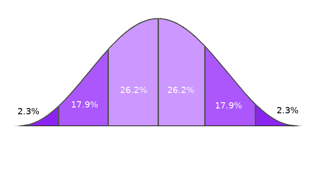
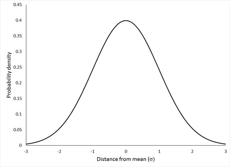
Normal distribution is the most commonly used distribution out of every distribution pattern out there. Even those who’ve never studied a page of elementary statistics in their life are bound to come across a lot of statistical data represented using this ‘bell-shaped’ distribution.
Normal distribution, also known as the Gaussian distribution, is a continuous probability distribution which is symmetric in nature. It represents the values across the curve in a manner such that the values are clustered around the peak and the curve tapers off towards the ends as we move further away from the peak.
This distribution creates a peak around the mean and the tapering at the either sides resembles the shape of a bell and hence this distribution is also called as a bell curve.
Normal distribution occurs widely in a lot of data related to real life and humans like height of people, educational test scores, IQ, health, salaries etc and hence is widely used by Government bodies in various fields of life.
The Probability Density Function for a normal distribution is given by the formula:
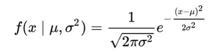
where µ = mean and σ = standard deviation
Hence, variation in the standard deviation shapes how the bell curve spreads out and the width of the normal distribution. Usually, standard deviation expresses the measure of variability. When the standard deviation is smaller, the bell curve is taller because the data is clustered around the mean more tightly. And similarly, when the standard deviation is larger, the bell curve is wider and the curve is flatter because the data is spread out away from the mean. The standard deviation also lets us predict the distance between the average and the observations.
In a normal distribution, the mean, median and mode coincide and are all equal with exactly half of values to the left of the mean and exactly half of the values to the right of the mean. Or an another way to say it is that in a normal distribution, half the population will be greater than the mean and half of the population is always be lesser than the mean. Also since, the normal distribution is symmetric in nature, the distribution cannot model data which is either skewed to the left or skewed to the right.
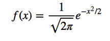
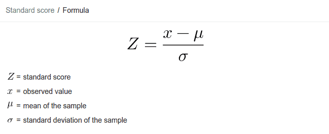
Standard Normal Distribution: Standard normal distribution is a special case of normal distribution in which the mean (µ) = 0 and standard deviation (σ ) = 1 which then simplifies the probability density function to
It is actually the normal random variable of a standard normal distribution that is called a Z Score which is subsequently used to studying the Z Table which let’s us study the values of the cumulative distribution function of the normal distribution. This let’s draw a lot of inferences and data from a normal distribution like the areas under a curve, p-value, distances of Z from the mean, confidence intervals etc. However, it is to be noted that the area under the curve is always equal to 1. To transform a normal random variable into a Z Score, we use the following equation:
Bernoulli Distribution
Another very commonly used probability distribution is the Bernoulli Distribution. Bernoulli Distribution is a discrete probability distribution. It is as easy to use and easy to understand distribution.
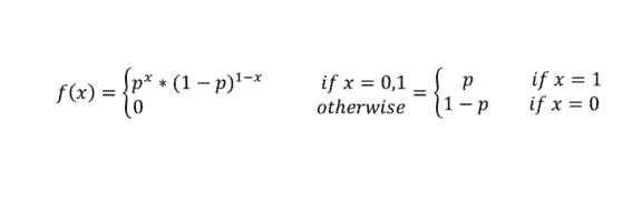
Definition: A Bernoulli Distribution is a type of distribution in which the random variable can only take a binary/boolean output. Meaning, a Bernoulli Distribution only has two possible outcome (referred to as ‘Success’ or ‘Failure’). 1 with probability p and 0 with probability (1 – p).
Hence the probability density function of the Bernoulli Distribution is given by the formula
To understand Bernoulli Distribution better or what a binary output means take the example of the coin toss that we discussed earlier. For a coin toss, in a single event, the only two possible outputs are either a Head or a Tail. There is no in between the either two outputs.
In case of a coin toss however, the probability of getting a heads = probability of getting a tails = 0.5. However, in Bernoulli Distribution the probability of the outcomes does need to be equal. Take for example the example below where the probability of failure (0) = 0.25 and the probability of success (1) = 0.75
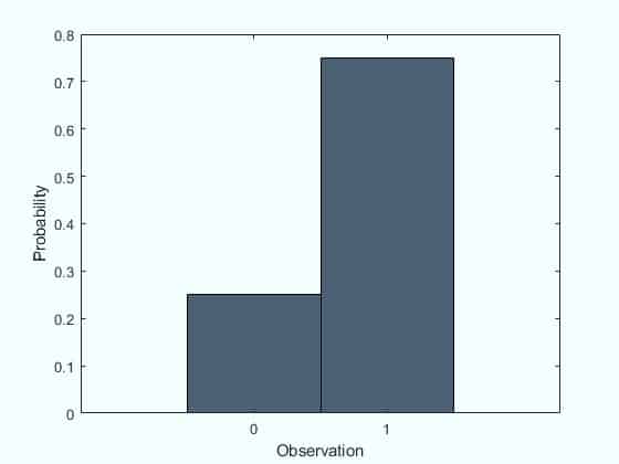
Please note that in Bernoulli Distribution the term ‘success’ and ‘failure’ only represent the occurrence of an outcome and are not to to be taken in literal sense of the words. So if a outcome you’re tracking occurs, it is noted as a success and if it does not occur, it is noted as a failure.
The outcomes in a Bernoulli Distribution are independent of each other. Meaning the outcomes are completely separate and do not influence each other in any way. A Bernoulli trial is an experiment with only two possible outcomes success and failure and where the probability of success stays the same every time that the experiment is performed.
Hence, the Binomial distribution and Bernoulli Distribution are closely related to each other. The number of successes in a Bernoulli trial is said to have a binomial distribution if each Bernoulli trial is independent. Or you can also frame the same statement as: the Bernoulli distribution is the Binomial distribution with n=1. We will take a more in depth look at the Binomial distribution in the next section.
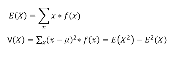
The expected value and variance in a Bernoulli Distribution is given as:
Binomial Distribution
The Binomial Distribution is closely related to the Bernoulli Distribution. While the Bernoulli distribution represents the outcome of a single Bernoulli trial as a ‘SUCCESS’ or ‘FAILURE’, the Binomial distribution represents the probability of success or failure of an experiment repeated multiple times or n independent Bernoulli trials.
Just like the Bernoulli distribution, the trials are independent for binomial distribution as well. Not only that, there are only two outcomes of each trial, either a binary 0 or 1 or a ‘Success’ or ‘Failure’ and these two facts stay the same for all n number of trials conducted in the experiment. Also the trials are identical, meaning the probability of the outcomes of success and failure is the same for all trials.
The probability density function for a Binomial distribution with n independent trials is given by the formula:
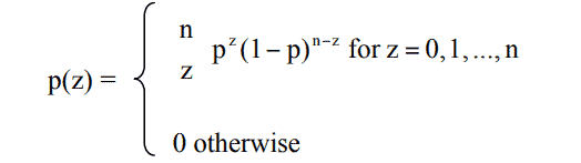
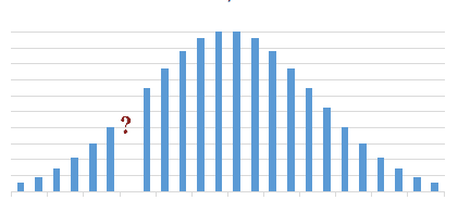
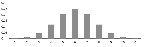
The Binomial distribution where the probability of the success is equal to the probability of failure, the distribution starts resembling the shape of a normal distribution or a bell curve as can be seen in the graph below.
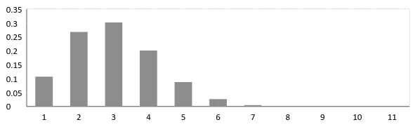
But it is not necessary for the binomial distribution to have the probability of success equal to the probability of failure, always. In which case, it can take a form like one below where the probability of success is not equal to the probability of failure
Uniform Distribution
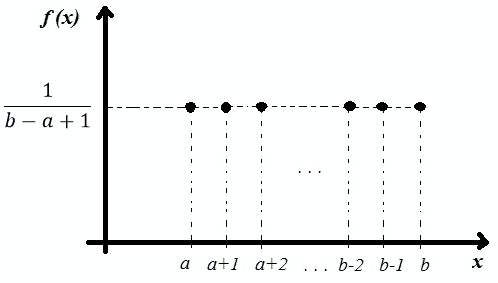
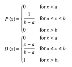
A Uniform distribution is defined as a distribution which has a constant probability. It is also called a rectangular distribution given the nature of the distribution graph usually which is a rectangle.
A Uniform distribution usually has only two parameters, the minimum and the maximum, represented by a and b, where:
- ‘a’ is used to denote the minimum
- ‘b’ is used to denote the maximum
And the distribution is denoted a U(a,b)
A uniform distribution can be both continuous or discrete in nature but the former is more commonly seen and used in statistics. In a discrete distribution however the finite sources of outcome are expressed using dots which still resemble a rectangular distribution as seen below
The P.D.F (Probability Density Function) and the C.D.F. (Cumulative distribution function) and for a continuous Uniform Distribution U(a,b) are given by the formula:
Poisson Distribution
A Poisson Distribution is a discrete probability distribution, named after the French Mathematician Simeon Denis Poisson, which expresses the the probability of events happening independently or at a constant mean rate within a fixed interval of space, time or volume. Meaning in simple words, the exact timing and count of events is random but the interval of time or space where these events occur is fixed.
The events occurring in a Poisson distribution are independent of each other and the occurrence of an event does not affect the next event which follows. For example, consider the number of books sold on each day of the week on an online website. The purchase of a book by a random reader or visitor of the site does not affect the other sales happening on the website. But at the same time one can predict both the average number of sales per week across the entire website and the pattern of higher or lower sales on a certain given day. Such a distribution of data obeys the Poisson Distribution.
The Probability Mass Function for a Poisson Distribution is expressed on a graphs as:
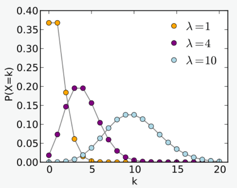
where λ = is used to denote the expected rate of occurrences as 1, 4 and 10 respectively and the horizontal axis accounts for the index k and the vertical axis accounts for the probability of k occurrences for λ
To calculate the probability of k occurrences over a time period, we use the formula
Where e is the Euler’s Number and X is the discrete random variable.
Exponential Distribution
Exponential distribution is continuous probability distribution that is widely used in statistics and real life data science. Exponential distribution is a probability distribution that let’s us model the time between two events in a Poisson point process. That is in simple words, it let’s us predict and model the time in between two events and thereby predict success, failure, waiting time etc until the next event.
The Exponential distribution is also known as the negative exponential distribution. It is closely related to the Poisson distribution and has wide usage in real life. Take the same example as talked previously in the Poisson Distribution sub-section. An exponential distribution in such a case would let model the time in between book sales.
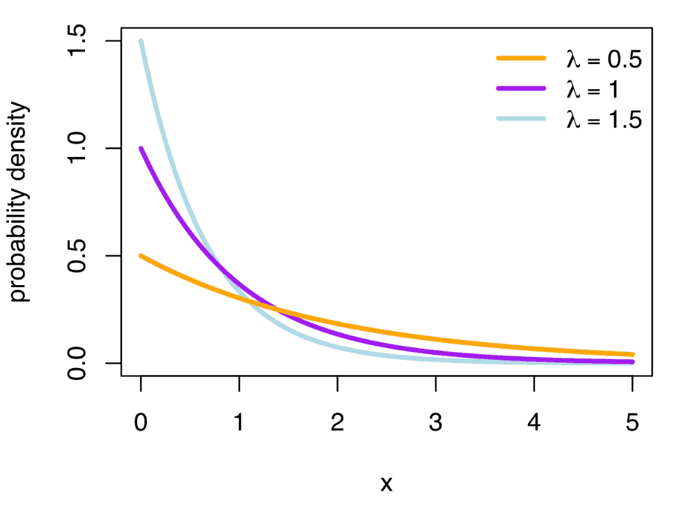
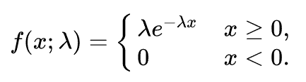
Probability Density Function of an Exponential Distribution
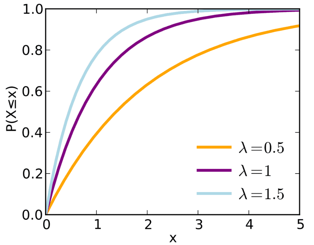
The Probability Density Function of an Exponential Distribution can be mapped on a graph for different values of λ as:
The same can be expressed as:
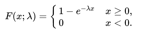
Cumulative Distribution Function of an Exponential Distribution
Whereas the Cumulative Distribution Function of an Exponential Distribution can be mapped as:
The same can be expressed as:
Relations between the commonly used Distributions
The commonly used distributions usually share a close relationship with each other such that one is a special case of other or a certain type of distribution resembles other under certain conditions. We will take a look at the relations between commonly used distributions below:
Poisson & Exponential Distribution: If an exponential distribution is followed for time between random events with a rate λ, then t the time period for the total number of events in that period follow a Poisson Distribution with parameter = λt
Binomial & Normal Distribution: If both p and q don’t tend to being too small and number of trials n tends to infinity or is indefinitely large, then normal distribution is a limiting form of binomial distribution
Poisson & Normal Distribution: If λ →∞ as a parameter for Poisson distribution then normal distribution is a limiting form of poisson distribution
Bernoulli & Binomial Distribution: Both Bernoulli and Binomial distribution independent trials and only two possible outcomes of binary nature i.e. True or False, Success or Failure or 0 or 1. A Bernoulli Distribution is considered to be a special case of Binomial Distribution with a single trial.
Poisson & Binomial Distribution: If np = λ is finite and the number of trials tend to infinity/too large and the probability of success of each trial same/indefinitely small/ p tends to 0 then the Poisson Distribution is a limiting case of binomial distribution
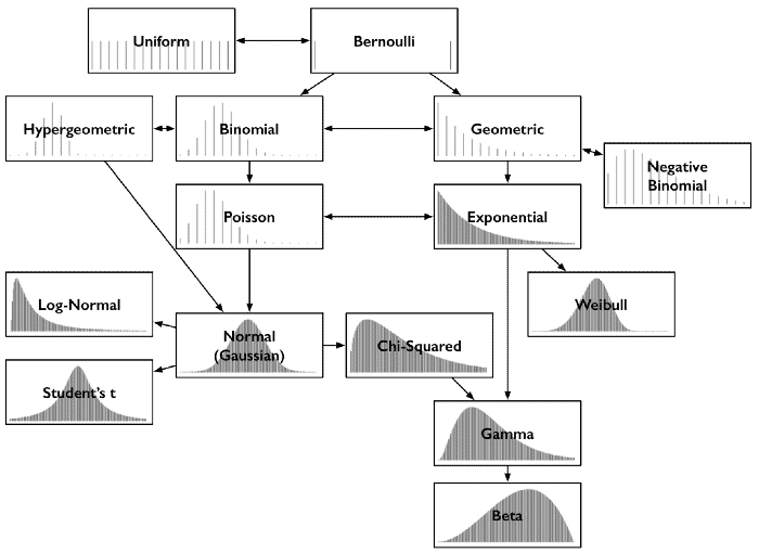
Other Types of Distribution
While we have studied six types of probability distributions up there, please know that they are not the only ones. There are different ‘families’ of distributions with each having multiple sub-types of distributions under them. Covering every single type of distribution is beyond the scope of this article because there are over a hundred of them. To name a few: Geometric and Hypergeometric distributions, Beta distribution, Yule-Simon distribution, Pearson distribution family, Student’s T Distribution, Hotelling’s T-squared distribution, F-distribution, Boltzmann Distribution, lognormal distribution, Rademacher distribution etc.
Instead a better approach is to learn the basic and most widely used distributions thoroughly which will let you understand the distributions related to it or derived similar to it more easily. For example, a thorough knowledge of the Gaussian distribution will let you easily pick up the Student’s T Distribution, Chi-squared Distribution and the Lognormal distribution.
References
- Encyclopedia of Mathematics. Probability Distribution https://encyclopediaofmath.org/index.php?title=Probability_distribution
- The Cambridge Dictionary of Statistics https://www.worldcat.org/title/cambridge-dictionary-of-statistics/oclc/161828328
- Basic Probability Theory https://www.worldcat.org/title/basic-probability-theory/oclc/190785258
- A Second Course In Probability http://people.bu.edu/pekoz/A_Second_Course_in_Probability-Ross-Pekoz.pdf
- Probability density function https://en.wikipedia.org/wiki/Probability_density_function
- Elementary Probability https://archive.org/details/elementaryprobab0000stir
- Probability Mass function https://en.wikipedia.org/wiki/Probability_mass_function
- Encyclopedia of Mathematics. Normal Distribution https://encyclopediaofmath.org/index.php?title=Normal_distribution
- Why are Normal Distributions Normal? https://aidanlyon.com/normal_distributions.pdf
- Univariate Distribution Relationship http://www.math.wm.edu/~leemis/chart/UDR/UDR.html
- Introduction to Modern Statistics “Binomial Distribution—Success or Failure, How Likely Are They?” https://books.google.co.in/books?id=KostAAAAIAAJ&pg=PA140&redir_esc=y
- CRC Standard Mathematical Tables and Formulae, 31st Edition (Advances in Applied Mathematics) 31st Edition by Daniel Zwillinger https://www.amazon.com/exec/obidos/ASIN/1584882913/ref=nosim/ericstreasuretro