What is Normal Distribution?
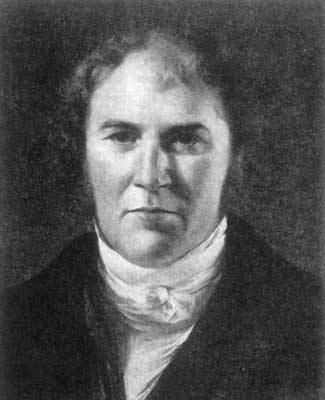
Normal Distribution also known as Gaussian Distribution (named after the German mathematician Carl Gauss who first described it) is a continuous probability distribution in which the occurrence of data is more clustered near the mean than the occurrence of data far from the mean. This characteristic lends the normal distribution a bell curve like shape which is symmetric about the mean. Normal distribution is one of the most common types of distribution patterns used in statistics and real life.
Examples of Normal Distribution
Example 1: Normal Distribution of Test Scores
A Normal Distribution can be observed by analyzing the test scores of students for any particular course. A large number of students will score the average score (say 65 out of 100), while a few will score near 50s or 80s and fewer will fail the test or get a perfect score. If the scores of these students were to be mapped on a graph, it would lend itself the shape of a bell curve.
Example 2: Normal Distribution of Weights of Newborn Babies
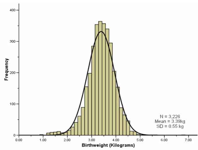
From the figure above we can observe that the average weight of a newborn baby is close to 3.5 kilograms and many of them weigh somewhere in between 3 kilograms to 4 kilograms. But as we move farther from the mean we find that very few babies weigh 2 kilograms or 5 kilograms and fewer weigh 1 kilogram or 6 kilograms. Such a distribution is said to follow the bell curve or a normal distribution pattern
Other common examples of normal distribution that we can observe around us on a daily basis are:
- Height of girls belonging to a certain age group.
- SAT or GRE scores.
- Salaries of employees working for the same organisation.
Normal Distribution Graph & It’s Characteristics
- The area under the Normal Distribution curve represents probability and the total area under the curve is 1.
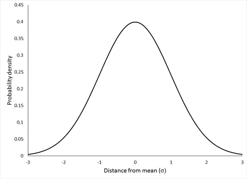
2. Normal distribution is symmetrical on both sides of the mean i.e. the values are evenly distributed to form identical halves on both sides of the mean.
3. For a normal distribution the mean, median and mode are equal
4. In a normal distribution graph, the further a value is from the mean, the less likely it is to occur and the ones that cluster around the mean are more likely to occur.
5. The tails of a normally distributed graph approach the x-axis but never quite really touch.
What is Probability Density Function?
Probability Density Function (PDF) is a statistical function in probability theory whose value in the sample space at any given point or sample, can be interpreted as providing a relative likelihood that the value of the random variable would equal that sample.
Probability Density Function determines the probability of a random variable to take a value bound between the given intervals. In statistics theory, PDF is popularly known for helping us calculate the probabilities associated with the random variables.
Probability Density Function Properties
Let us consider a continuous random variable x with density function f(x), then the Probability Density Function should satisfy the following conditions:
- The density function is always non-negative i.e. f(x) > 0, for all possible values of x
- The area under the curve is equal to 1, i.e. ∫f(x)dx = 1 (x belongs to ∞, −∞)
Probability Density Function of Normal Distribution
A Probability Density Function (PDF) for a Normal Distribution with a continuous random variable x, with mean μ, variance σ 2 and standard deviation σ is given as:
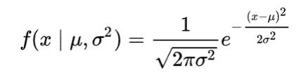
The mean of a Normal Distribution is the centroid of the Probability Density Function and the standard deviation σ is a measure of the dispersion of the several random variables around the mean. Since normal distributions are defined by the mean and standard deviation, let us have a more in depth look at both of them.
What is Mean?
In a normal distribution, the mean is the central tendency & peak of the distribution around which most of the values cluster around. Mean is proven to be an important measure in study of probability theory because it incorporates the entire data values obtained from population and gives us an idea of the behavioural patterns of the dataset.
For example, to find out how much a typical New Yorker pays as monthly rent ‘on an average’, the best way is to find a dataset that holds the information about the monthly rents paid by individuals living in New York, adding all the rent values and dividing it by number of individuals we included in this research.
Similarly when it comes to more complex datasets, to find the mean we add up all the data values and divide it by size of the dataset. It is represented by the symbol μ (Greek alphabet ‘Mu’).
If we plot a dataset where the values are normally distributed, we end up with something known as Normal Curve (Bell Curve), where peak of the curve represents our mean value and the dataset represents a Normal Distribution.
What is Standard Deviation
A Standard Deviation is a measure of how spread out the data values are below the curve and is represented by the symbol σ (Greek letter ‘sigma’). It represents the dispersion of the data values belonging to a dataset with respect to its mean. Meaning the smaller the standard deviation, the closer the data values are to the mean and the higher the standard deviation, the further away & spread out the data values are from the mean.
There are two types of standard deviations namely: Sample standard deviation and population standard deviation. Given by the formulas:
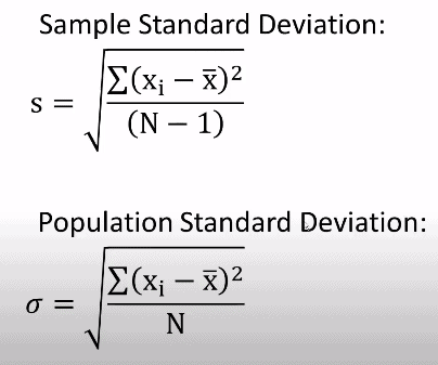
where
σ – population standard deviation
S – sample standard deviation
N – size of the population
xi – each data value from the population
x̅ – population mean
Standard Deviation and the 68-95-99.7 Rule
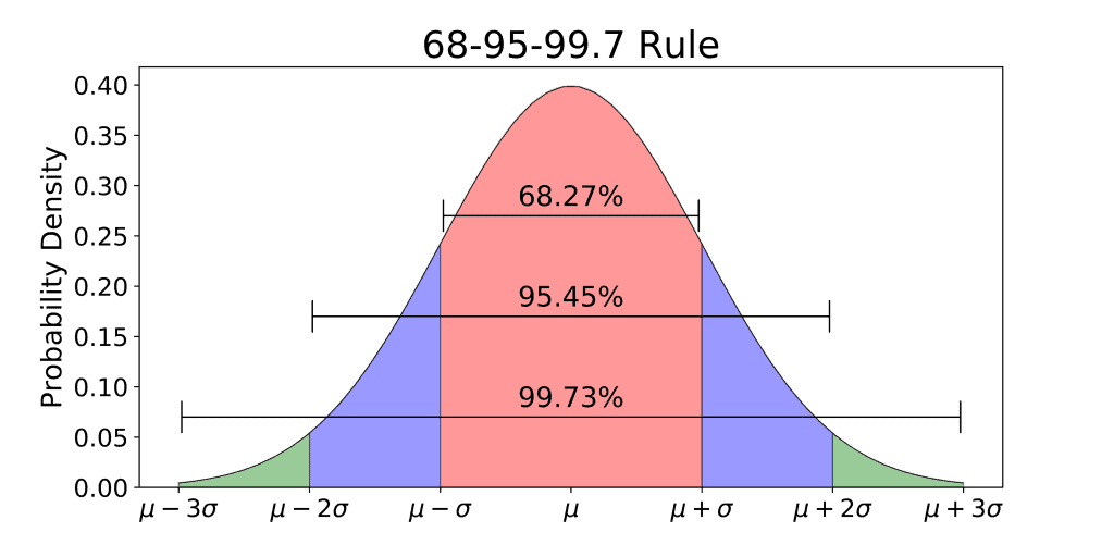
The 68-95-99.7 Rule, as known as the Empirical Rule for normal distributions, coined by Abraham De Moivre, states that for a standard normal distribution:
- 68% of all the values fall within one standard deviation from the mean
- 95% of all the values fall within two standard deviations from the mean
- 99.7% of all values, or nearly all values, fall within three standard deviations from the mean
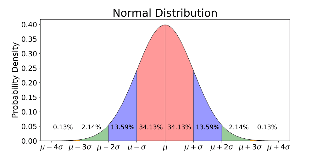
Since the normal distribution is symmetric in nature, the Empirical rule can also be demonstrated as:
Normal Cure | Bell Curve
The Normal Distribution curve is also known as the normal curve or the ‘Bell Curve’. The name originates from the fact that a curve used to depict Normal Distribution resembles the shape of a bell. The bell curve is symmetrical as half of the data will fall to the left of the mean while the other half will fall to the right. The terms normal distribution, normal curve and bell curve are often used interchangeably in statistics.
Uses of Normal Distribution
It is observed that many natural phenomena follow ‘Bell Curve’ type of pattern of data and probability distribution. Data scientists observe the existence of normally distributed patterns of data in most common fields where data is heavily used like business, medical analysis, private organizations and in government bodies. To name a few examples:
- We observe Normal Distribution being abundantly used by the manufactures to understand the inclination of its consumers towards a particular item. This helps them understand consumer psychology and also helps them enhance the consumer-buyer relationship.
- Universities may use the Normal Distribution to design their tests.
- Insurance companies predict the probability of accidents including various parameters about the insured individual to provide them with premium.
- Drug manufacturing organization use Normal Distribution to validate their clinical research and improve the medications to cause lesser side effects.
- Marketing departments will collect information on likelihood of demand of their products at different price points to determine a correct pricing.
- Electronic circuits with weak signals (radio receivers or microphone preamps) are sensitive to thermal noise and these signals resemble a Normal Distribution. Hence, calculating factors such as “bit error rate” or “false alarm rate” becomes easier.
Standard Normal Distribution
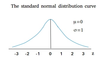
A Standard Normal Distribution (SND) is a Normal Distribution with mean zero and standard deviation of 1. It is centered at zero (mean) and has intervals spaced 1 standard deviation apart on both sides of the mean.
Any Normal Distribution with any mean and any standard deviation can be converted into a Standard Normal Distribution, where you have mean zero and standard deviation 1, through a conversion known and Standardization.
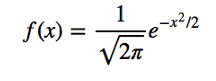
Probability Density Function formula for Standard Normal Distribution
The probability density function for a standard normal distribution with a mean (µ) of 0 and standard deviation (σ ) of 1 simplifies to:
Z-Scores or Standard Scores
Each number on the horizontal axis of a Standard Normal Distribution curve corresponds to Z-Score also most commonly known as a Standard Score.
Z-Score tells us how many standard deviations an observation is from the mean μ. For example, the Z-Score of 2.5(positive Z-Score) indicates that the value is 2.5 standard deviations away to the right of the mean, whereas a Z-Score of -1(negative Z-Score) indicates that the value is 1 standard deviation away to the left of the mean and if a Z-Score is equal to 0, then it indicates that the Z-Score is equivalent to mean.
The benefit of Standardization is that with the help of a Z-Score table we can easily calculate exact areas for any given normally distributed population with any mean or standard deviation and it also enables us to compare two scores that are from different samples which may have different means and standard deviations.
For Standardization or to obtain the standard score, we use the ‘Z-Score’ formula:
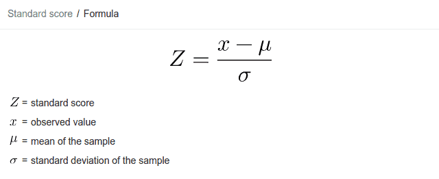
Z Table or Standard Normal Table
A Z-Score allows us to calculate how much area that specific Z-Score is associated with and we can find out that exact area with help of ‘Z-Score Table’ also known as ‘Standard Normal Table’.
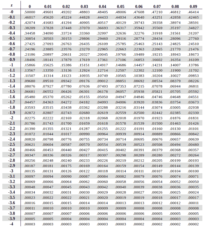
The values that are less than mean (zero), correspond to a negative score in Z-Table and lie to the left of the mean as observed in the figure above. To calculate the Z-Score of these negative values we refer Negative Z Score Table.
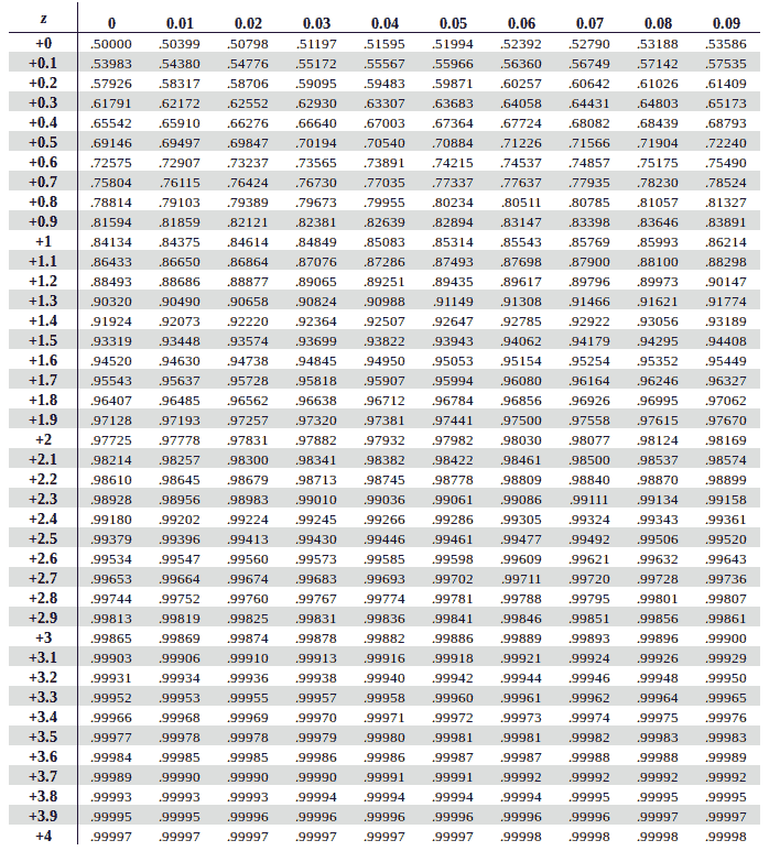
Similarly, the values that are greater than mean (zero), make positive score in Z-Table and lie to the right of the mean on graph. Hence, to calculate the Z-Score of these positive values we refer the Positive Z Score Table.
How to use the Z-Table
Let us understand how to use Z-Score formula and Z-Table with the help of few examples:
Example 1: The test scores of 50 students in a class is normally distributed with a mean = 65 and a standard deviation = 8. What proportion of students score less than 46.
Solution: Let X denote proportion of students scoring less than 46, P (X < 46).
Using Z-Score formula we get,
= P (Z < X – μ / σ)
= P (Z < 46 – 65/ 8)
= P (Z < -2.37)
Therefore, P (X < 46) = P (Z < -2.37)
To map the same on the Z-Table, we need to choose the respective Z-Table (negative or positive) based on whether our Z Score is negative or positive. In our case, the Z Score is -2.37 so will use the negative Z Table.
To find area under the curve for -2.37, first we traverse in horizontal direction along the leftmost column along the Y-axis to find the value of the first two digits of Z Score (-2.3 based on our example)
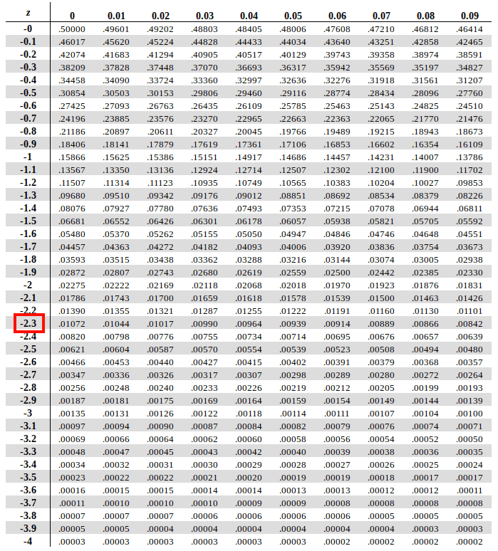
After that we need to run alongside the X-axis of topmost row to find the value of digits at the second decimal position (0.07 based on our example)
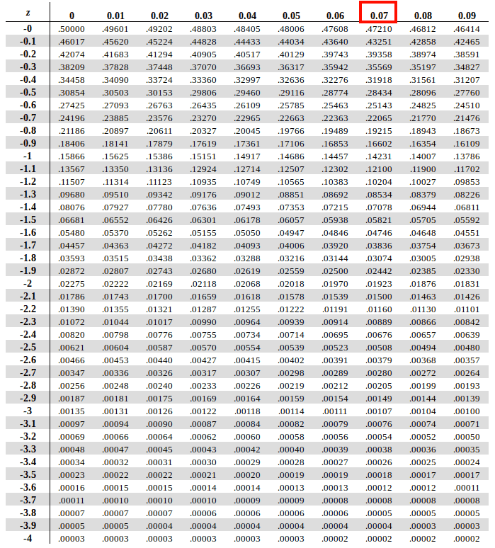
Now map these two values on the Z-table and find the intersection of the row of first two digits and column of the second decimal value in table. And voila! the intersection of the two is our answer.
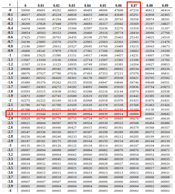
According to the Z-Score table, we get Therefore P(x<46) = P(Z<-2.37) = 0.00889, which indicates only 0.88 % (0.00889 X 100) of students score less than 46.
Example 2: The test score of 50 students in a class is normally distributed with mean 65 and a standard deviation of 8. What proportion of students score more than 75.
Solution: Let X denote proportion of students who score more than 75, P (X > 75).
Using Z-Score formula we get,
= P (X- μ/ σ > X – 65 / σ)
= P (Z > 75 – 65/ 8)
= P (Z > 1.25)
i.e. P (X > 75) = P (Z > 1.25)
According to the Z-Score table, we get P (Z < 1.25) = 0.8944 (area to the left of the Z-Score), this indicates 89.44% of students scored less than 75.
But we need to find the proportion of students who scored more than 75, P (Z > 1.25) which lies to the right of the calculated Z-Score.
The most important thing to understand when calculating area under the curve to the right of Z-Score is,
Area (on right) = 1 – Area (on left)
Therefore, P (Z > 1.25) = 1 – 0.8944 = 0.1056
Only 10.56% of students scored more than 75 on a test.
History of Normal Distribution
The credits for the discovery of the normal distribution are not unanimous. Some authors attribute the credit to Abraham de Moivre and some authors attribute the credit to Carl Friedrich Gauss.

De Moivre published the study of coefficients in the binomial expansion of (a+b)n in the second edition of his textbook on probability ‘The Doctrine of Chances’ in 1738.

Whereas Gauss introduced normal distribution along with other important mathematical concepts like the method of least squares in his monograph published as “Theoria motus corporum coelestium in sectionibus conicis solem ambientium“. Hence, the normal distribution has also been interchangeably known as the Gaussian Distribution over the years.

Pierre-Simon Laplace is also credited with making significant contributions to the normal distribution since he was the first to pose the problem of aggregating observations. However, it led him to crafting his own double exponential distribution as a solution which is known as the Laplacian distribution. It was also Laplace and not Gauss who proved the central limit theorem, which acts as a theoretical base to the normal distribution.
A lesser known fact is that an Irish mathematician by the name of Robert Adrain published in the year 1809 two derivations of the normal probability law completely independent from Gauss’s work which was only later rediscovered by the Cleveland meteorologist Cleveland Abbe in the year 1871.
Right from the coining of the normal distribution, it has been known by various different names. Following were the names interchangeably used for the normal distribution to name a few:
- Normal probability law
- Normal distribution
- Gaussian distribution
- Gaussian law
- Laplace’s second law
- Normal curve
- The law of facility of errors
- Bell curve
- The law of error
Gauss said he used the term ‘normal’ in reference to the ‘normal equations’ implying the technical meaning of ‘orthogonal’ and not ‘usual’. This led to confusion because many statisticians, students and teachers alike, have used the ‘normal’ as an adjective, implying it as ‘usual’, ‘common’, ‘typical’ and hence ‘normal’. It was actually Karl Pearson in 20th century who gave the term ‘normal’ it’s rightful designation for the distribution and the way it was intended to be and popularized it.
References:
- http://jeff560.tripod.com/s.html
- https://aidanlyon.com/normal_distributions.pdf
- https://en.wikipedia.org/wiki/The_Doctrine_of_Chances
- https://encyclopediaofmath.org/wiki/Normal_distribution
- https://projecteuclid.org/euclid.aoms/1177728796
- https://www.jstatsoft.org/article/view/v011i04
- https://www.ztable.net/how-to-create-a-z-score-table/