Degrees of Freedom Definition
The degree of freedom is defined as the number of independent values that can vary in any analysis without breaking the constraints of the analysis. In the estimation of a statistical parameter, this can be described as the number of values that can vary. This is an essential concept in statistics including regression analysis, hypothesis test, and parameter estimation. It is the amount of independent information that goes into the calculation of an estimate.
Symbol: ( Df ) is the commonly used abbreviation for the degree of freedom.
What is Degrees of Freedom?
Degrees of freedom indicates the values in a sample test that can vary in the estimation of parameters. It can be thought of as a mathematical restriction that should be implemented while estimating a population parameter by estimating others. These variations are in such a way that the constraints of the test are not compromised. It is the freedom of variables to vary or change while strictly staying within the constraints. If there are no rules, limitations, or patterns to be followed, then all the independent values have the freedom to vary. Here the degree of freedom has the value of the sample size.
Degrees of freedom often have applications in the calculation of population parameters from the sample statistics. The degree of freedom is not precisely the sample size. If we are to take a sample of size n, then typically, the degree of freedom for this sample will be the sample size minus 1. That is, n-1 independent values in the sample that is being considered have the freedom to vary.
Degrees of freedom Df = N – 1
Where N is the number of independent values taken for the sample.
The degree of freedom is a positive whole number. It can also be zero in the case of a sample with only one individual value.
Example of Degrees of Freedom
Let us understand the degrees of freedom more clearly by taking an example.
Example 1: Let us say that a girl has five pair shoes. She could wear any of them according to her preference. A constrain is placed on her that she has to wear a different pair of shoes each day for the next five days.
On the first day, she could choose any of the five pair of shoes. The next day she could choose all but the shoes she wore the previous day. Hence she could choose from the remaining four. This could be continued until the last day, where she could wear the only remaining pair. On the fifth day, there is no choice left for her. She must wear the last shoes. Unlike the previous days, she couldn’t vary her choice. This arises due to the constraint that she must not choose the used shoes again. Hence we could say that for 5-1 = 4 days, she had the chance to vary the shoes. Therefore 4 is the degree of freedom in this case.
Example 2: If we are to take an example statistically, we can take six integers. Now, if there are no conditions or constraints attached, these six integers are free to take up any values. Hence the degree of freedom, in this case, will be 6.
Now, say that the mean of the 6 value should be 4. This becomes the constraint for the test. We are free to choose the elements but the mean value should be 4.
We can take some random values for the sample. Let’s say we choose the first five values
First five Values = 1, 2, 3, 4, 5
By taking its sum, we get 1 + 2 + 3 + 4 + 5 = 15
For the mean to be equal to 4, the sum of the values must be equal to:
N * mean = 6 * 4 = 24
For this to be kept true, the sixth element of the sample must be equal to 24 – 15 = 9.
We cannot pick the sixth element randomly once we fix the other elements. We had the liberty to choose any number we wished for the first five elements but not for the sixth one.
Hence the degree of freedom is 6 – 1 = 5
Why do we have to subtract one from the number of elements?
If there are any constraints that should be obeyed, we have to subtract one from the sample size n. If no constraints are present, then the sample size itself is the degree of freedom. However in most cases in real life, at least one constraint will be placed if not more. Parameter estimation could not be carried out by defining or stating nothing. Hence the subtraction of one for analyzing the degree of estimation.
As it is observed from the previous examples, we can vary all the elements in the sample but one. The last element taken should be in such a way that it must not break the constraint. For this, we have to fix the other elements as well. Once all the elements except one are fixed, it is necessary for the last element to uphold the conditions that are set for the sample. Hence we have no choice but to select a particular value for this. It is chosen not randomly but precisely. Therefore we conclude that the last element has no degree of freedom. Hence we subtract this from the number of elements.
Degrees of Freedom For Z-Test and T-Test
Z-tests use standard normal distribution for the hypothesis test to calculate the significance of the results of an experiment. Unlike other distributions which change their shape as the number of observations vary, the standard normal distribution does not change with number of observations.
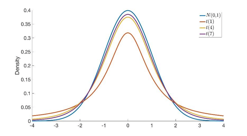
Whereas T-tests use t distribution for the hypothesis test to calculate the significance of the results of an experiment and unlike the standard normal distribution, the T-distribution changes based on the number of observations as well as the degrees of freedom.
Hence, while the Z-test does not depend on the degrees of freedom, the T-test does depend on the degrees of freedom. For an one-sample t-test with n sample size, the degree of freedom will be n – 1. The degree of freedom largely defines the shape of the t-distribution in every hypothesis test and the distributions are designed this way to reflect the same.
Meaning, as Df is closely related to the sample size, the t distribution graph is largely affected by the Df. if the degree of freedom decreases, the graph will have thicker tails. This is because the sample size will be small if the degree of freedom is decreased. This will also show the uncertainty in the result associated with a lower sample size in an experiment. It is always recommended to increase the sample size to reduce uncertainty and errors. Whereas as the sample size increases to infinity, the t-distribution graph converges to a standard normal distribution graph
Degrees of Freedom for the Chi-Square Test of Independence
This is another type of hypothesis test where we find the relationship between categorical variables. Categorical variables are variables based on a particular characteristic and have values for a countable number of distinct groups. For example, a university major is a categorical variable that can have values like medicine, law, physics, engineering, etc.
For this test, we create a Chi-Square table where each cell represents the frequency observed for each combination of categorical variables. Degrees of freedom can be defined as the number of cells in the Chi-Square table that can vary before the calculation of all other cells. The totals in the margin of the table are the constraints for the variables.
Generally, for a Chi-square table with n rows and m columns, the rule for the calculator of degrees of freedom is ( n – 1 ) ( m – 1 ).
The following table is a 2X2 Chi-square table.
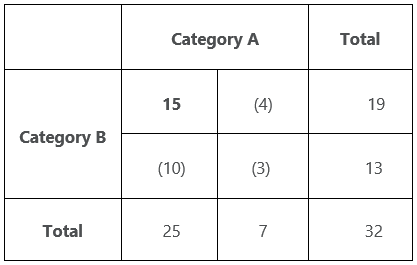
The total values will be the constraints in our experiment and it will be already given. Also, say that we fix one value, 15 in the first cell. Now, we cannot choose whichever value we like for the cells in which the values are given in parentheses. We have to make sure that the total sum of the values in each row and column corresponds to their given values. Hence the remaining three cells have values that are fixed by taking 15 as the first cell value. therefore, the Df for this table will be 1. That is, we can only choose one value randomly.
Also, as per our rule, the degree of freedom = (n -1) (m – 1) = (2 – 1) (2 – 1) = 1.
Here too, the shape of the graph in the calculation of p-value is affected by Df